What Are the Different Types of Fiber Misalignment?
In optical communication systems and photonic device manufacturing, getting light from one fiber into another sounds simple in theory. A single-mode fiber core measures roughly 8 to 10 microns across, about one-tenth the width of a human hair. Even sub-micron positioning errors between two fiber ends can wipe out half the transmitted signal. This is why a motorized translation stagewith sub-micron resolution is indispensable in any optical system that uses a fiber coupler. Understanding exactly how fibers can be misaligned is the starting point for designing assembly processes that work, whether you are packaging laser diodes, assembling optical transceivers, or building silicon photonic chips.
Fiber misalignment falls into four fundamental categories: lateral offset, angular tilt, longitudinal gap variation, and rotational error. Each type reduces coupling efficiency differently, and in real systems they almost never occur in isolation, which is why active multi-axis correction with a fiber coupling stage is essential.
This article walks through each fiber misalignment type, explains what causes it and how much loss it introduces, and shows how precision positioning equipment turns these sub-micron challenges into repeatable manufacturing processes.
How fiber misalignment affects coupling efficiency
Every type of fiber misalignment reduces the overlap between the mode field diameters of the two fibers, which directly lowers the fraction of transmitted optical power.
The physics is straightforward: for light to travel from one fiber into another, the two mode fields must overlap as completely as possible. Any deviation from perfect alignment shrinks that overlap integral, producing what is known as insertion loss. In a single-mode fiber coupler, the relationship between fiber misalignment and loss is highly nonlinear. A 1-micron lateral offset might produce 0.5 dB of loss in one configuration and 3 dB in another where the mode field diameter is smaller.
This sensitivity explains why active alignment, where the position of one fiber relative to another is continuously adjusted while measuring real-time optical power, has become the dominant approach in high-yield optical assembly lines. Passive alignment, which relies on mechanical datums and pre-machined features, usually requires live feedback to achieve sub-micron repeatability.
Mode field diameter and alignment tolerance
A larger mode field diameter makes a fiber more tolerant to lateral and angular errors because the overlap integral changes more slowly. This is why multimode fibers, with core diameters of 50 or 62.5 microns, are far easier to align than single-mode fibers. The trade-off is bandwidth: larger cores support more modes, which creates modal dispersion and limits transmission distance.
For single-mode fibers at 1550 nm, the standard mode field diameter is around 10.4 microns. The alignment tolerance, defined as the misalignment that produces 1 dB of excess loss, is typically under 1.5 microns for lateral offset and under 0.3 degrees for angular tilt. These numbers drive the specification of equipment used in optical transceiver coupling and silicon photonics packaging.
Lateral misalignment (axial offset)
Lateral misalignment, also called axial offset or radial misalignment, is the most common and most loss-sensitive type of fiber misalignment, occurring when the two fiber cores are parallel but offset perpendicular to the optical axis.
Imagine two cylinders that should be end-to-end but are instead shifted sideways so their centerlines do not coincide. In a single-mode fiber with a 10.4-micron mode field diameter, an offset of just 1 micron can introduce more than 0.5 dB of insertion loss. At 2 microns, the loss can exceed 2 dB. This steep penalty curve means lateral alignment is the first thing any fiber alignment stage must correct.
Causes of lateral offset
Cause
Typical offset range
Impact severity
Mechanical tolerance in connector ferrules
0.5 to 2 μm
Moderate
Thermal expansion mismatch between fiber and substrate
0.1 to 0.5 μm per °C
Cumulative
Inaccurate pick-and-place during die bonding
1 to 5 μm
High
V-groove width variation in passive alignment
0.2 to 1 μm
Process-dependent
Epoxy shrinkage during curing
0.5 to 3 μm
Can shift post-cure
In production environments, lateral offset rarely has a single cause. Epoxy shrinkage during cure can undo a perfect pre-cure alignment. Thermal gradients across an optical fiber alignment system can drift a precisely positioned fiber by microns over minutes. The cumulative effect is why closed-loop active alignment has become standard practice for high-value optical assemblies.
Correcting lateral offset with precision stages
A motorized linear stage with sub-micron resolution is the most direct way to correct lateral misalignment. The stage drives one fiber in the plane perpendicular to the optical axis while an optical power meter provides live feedback. The alignment algorithm, typically a hill-climbing or spiral search, finds the position that maximizes coupled power.
For single-axis adjustments, a manual positioning stage with a fine-pitch leadscrew and micrometer drive can achieve 0.5-micron resolution. But when both X and Y axes need simultaneous optimization, as is almost always the case, a multi-axis translation stage or an XYZ motorized stage becomes necessary. The search space grows quickly: a naive 2D raster scan at 0.1-micron resolution over a 10 by 10 micron window requires 10,000 power measurements.
Angular misalignment
Angular misalignment occurs when the two fiber end faces are not parallel, with one fiber tilted relative to the other by a small angle, causing the emitted light cone to strike the receiving fiber core at an angle that reduces the overlap integral.
Even a tilt of 0.5 degrees can introduce over 1 dB of loss in single-mode systems. The loss mechanism is geometric: the tilted fiber emits light in a direction that does not fully enter the acceptance cone of the receiving fiber. The smaller the numerical aperture, the more sensitive the coupling is to angular errors.
Angular misalignment matters most in connector-based systems and in free-space coupling configurations, for instance, between a lensed fiber and a photonic integrated circuit grating coupler. In these setups, the fiber is not butt-coupled; a small air gap or lens system separates the two ends, and any tilt is magnified by the optical path length.
Sources of angular error
Angular errors come from three main sources: cleave angle variation, where the fiber end face is cut at an angle apart from 90 degrees to the axis; mount tilt, where the fiber holder or V-groove is not perpendicular to the optical axis; and goniometric stage misalignment, where the rotation axis of the alignment mechanism does not match the intended pivot point.
A poorly executed cleave can leave a 1-degree angle on the fiber end face. In a butt-coupled configuration, the cleave angle directly becomes a 1-degree angular misalignment. For this reason, production-grade cleavers specify end-face angles to within 0.5 degrees or better.
In an active alignment stage setup, angular correction is handled by a goniometer or a tip-tilt platform. These devices rotate the fiber around a pivot point near the fiber tip, allowing angular adjustment without introducing large lateral offsets. A well-designed 6-DOF positioning stage can decouple angular and lateral adjustments, which speeds up alignment convergence significantly.
Longitudinal misalignment (gap variation)
Longitudinal misalignment refers to an unintended gap between the two fiber end faces along the optical axis, either too large, causing beam divergence loss, or too small, risking physical contact damage to the fiber end faces.
The beam exiting a single-mode fiber diverges with a half-angle determined by the numerical aperture. For a standard SMF-28 fiber at 1550 nm, the divergence half-angle is roughly 5 degrees. Over a 10-micron gap, the beam expands by less than 2 microns, negligible for most systems. But at 50 microns, the beam diameter at the receiving fiber face can be noticeably larger than the mode field diameter, producing measurable insertion loss.
At the other extreme, a zero or negative gap can damage fiber end faces, especially in connectorized systems that are repeatedly mated. Physical contact connectors are designed to maintain a controlled spring force that keeps two polished end faces touching without exceeding the compressive stress limit of the glass.
Gap control in coupling stations
Most fiber coupling stage configurations include a Z-axis for controlling longitudinal position. The initial approach is typically done at higher speed with a coarse stage or a motorized linear stage operating in open-loop mode. Once the fiber tips are within roughly 20 microns of each other, the system switches to a finer step size and may use a contact-detection algorithm, monitoring for a sudden change in reflected power or a force sensor trip, to stop at the optimal gap.
In production environments, the Z-axis also handles the epoxy dispensing step. After alignment, one fiber must typically be retracted slightly, adhesive applied, and then the fiber re-advanced to the previously recorded optimal position. A high-precision motorized stage with bidirectional repeatability under 0.5 microns is essential for this sequence.
Rotational misalignment
Rotational misalignment is specific to polarization-maintaining fibers and other non-circularly symmetric fiber types, occurring when the angular orientation of the fiber cross-section around the optical axis does not match between the two fibers.
For standard single-mode fibers with circular cores, rotational alignment is irrelevant. Rotating a circular core around its center changes nothing about the optical coupling. But polarization-maintaining fibers, which have stress rods or an elliptical core to create birefringence, must be rotationally aligned so the slow axis of one fiber matches the slow axis of the other. A rotational error of just a few degrees can degrade the polarization extinction ratio from 30 dB to under 20 dB.
The same constraint applies when coupling to edge-emitting laser diodes, which produce an elliptical output beam. The major axis of the ellipse must align with the major axis of the receiving fiber’s mode field or with the input waveguide of a photonic chip. This is a common challenge in laser diode-to-fiber coupling stage applications.
Rotational alignment methods
Rotational alignment is handled by a rotary stage integrated into the fiber holding assembly. For silicon photonics alignment applications, where edge couplers are often polarization-sensitive, the rotary axis is scanned while monitoring both insertion loss and polarization-dependent loss. The optimal angle is the one that minimizes both.
Some optical transceiver coupling machine setups use image-based rotational pre-alignment. A side-view camera images the fiber and the chip edge, and a vision algorithm determines the rough angular orientation before the active alignment loop begins. This hybrid approach, using vision for coarse alignment and power feedback for fine alignment, reduces total cycle time.
Combined misalignment in real-world systems
In any real optical assembly, multiple types of fiber misalignment occur simultaneously, and their effects on coupling loss are not simply additive. Cross-coupling between axes makes optimization a genuinely multi-dimensional problem.
Consider a practical case: a fiber is being aligned to a photonic chip edge coupler using a multi-axis alignment stage. The initial placement, done by a pick-and-place machine, leaves the fiber with roughly 5 microns of lateral offset, 1 degree of angular tilt, and 20 microns of longitudinal gap. The operator, or the automation routine, must now optimize all six degrees of freedom.
The challenge is that correcting one axis often disturbs another. Reducing angular tilt by rotating the fiber around its tip also produces a lateral shift if the pivot point is not exactly at the fiber end face. Closing the longitudinal gap changes the beam diameter at the receiving plane, which in turn changes the optimal lateral position. These cross-axis effects are why sequential single-axis optimization often converges to a local maximum rather than the global optimum. A good fiber coupler alignment setup accounts for these interactions from the start.
Multi-axis optimization strategies
Optimization method
Axes handled
Typical convergence time
Suited for
Sequential hill-climbing (axis by axis)
2 to 3
30 to 90 seconds
Low-complexity single-mode coupling
Spiral search (2D raster)
2
10 to 30 seconds
Lateral-only, high-speed production
Gradient ascent (multi-axis simultaneous)
4 to 6
5 to 20 seconds
High-volume transceiver packaging
Simplex / Nelder-Mead
3 to 6
15 to 60 seconds
Robust, handles noisy power readings
Machine learning-guided search
4 to 6
0.5 to 5 seconds
Silicon photonics high-throughput lines
The trend in high-volume optical communication coupling alignment is toward gradient-based multi-axis optimization running on a high-precision motorized stage platform. The alignment algorithm moves all available axes simultaneously in the direction that maximizes the gradient of coupled power. When the system is well-calibrated, meaning the coordinate system of each axis is known relative to the others, convergence to better than 0.1 dB of optimal coupling can occur in under 5 seconds.
How precision alignment stages correct fiber misalignment
Precision alignment stages correct fiber misalignment by providing independently controllable motion along each axis where fiber misalignment can occur, with nanometer-level resolution and sub-micron bidirectional repeatability.
The core requirements for an optical fiber alignment system stage are straightforward in concept but demanding in specification: travel range sufficient to cover initial placement errors, typically tens of millimeters for coarse approach and tens of microns for fine alignment; resolution fine enough to optimize coupling to within 0.05 dB of the theoretical maximum, typically 10 to 50 nanometers for the fine axes; and stability good enough to hold that position through epoxy curing, with drift under 50 nanometers over 5 to 10 minutes.
Stage architecture for typical coupling applications
For single-mode fiber-to-fiber coupling, a minimal setup includes three linear axes: X and Y for lateral correction and Z for longitudinal gap control. This is often built from a stack of manual translation stage units for prototyping or from motorized linear stage components for production.
Adding angular correction requires tip-tilt stages or goniometers, bringing the axis count to five. A full 6-DOF positioning stage adds a rotary axis for polarization alignment. This is the standard configuration for silicon photonics wafer-level testing, where each die on a 300-mm wafer needs to be optically probed with sub-micron precision.
Drive technologies and their trade-offs
Drive type
Resolution
Repeatability
Speed
Best use case
Manual micrometer
0.5 to 1 μm
1 to 2 μm
N/A
R&D, low-volume prototyping
2-phase stepper motor
0.1 to 0.5 μm
±0.5 μm
Moderate
General-purpose automated alignment
5-phase stepper motor
0.05 to 0.1 μm
±0.1 μm
Moderate
High-resolution coupling stations
Linear motor (direct drive)
5 to 50 nm
±50 nm
High
High-throughput transceiver packaging
Piezo nanopositioner
<1 nm
±5 nm
Very high
Nano-alignment, PIC probing
A 5-phase stepper motor stage strikes a balance between resolution, cost, and complexity for most fiber coupler alignment applications. The five-phase design reduces vibration during low-speed moves compared to two-phase motors, which matters when aligning to a power reading that fluctuates with mechanical vibration. At the high end, direct-drive linear motors with optical encoder feedback can achieve closed-loop resolutions of 5 nanometers, which is overkill for most fiber alignment tasks but useful for waveguide-to-waveguide coupling in photonic integrated circuits.
Closed-loop vs. open-loop control
Any stage used for active alignment must operate in closed-loop mode, where an encoder or interferometer measures actual position and the controller corrects for leadscrew backlash, thermal drift, and other error sources. Open-loop stepper motor stages can lose steps under high load or during rapid direction reversals, producing an accumulated position error that the alignment algorithm cannot distinguish from a genuine power drop.
A precision linear stage with a linear encoder offers direct position feedback at the point of motion, eliminating leadscrew-related errors entirely. This is the preferred approach for production lines where repeatability across thousands of coupling cycles matters more than initial hardware cost. For teams specifying a fiber coupler alignment station, closed-loop control on all fine axes is a practical minimum.
Key considerations for selecting an alignment stage system
The most important factor in selecting an alignment stage system for fiber coupling is matching the stage configuration to the coupling geometry: the number of degrees of freedom that actually need correction, the required resolution in each axis, and whether the process is manual or automated.
Engineers evaluating options for their optical assembly line should look at several practical factors beyond the data sheet. The first is thermal stability: a stage that moves 50 nanometers for every degree Celsius of ambient temperature change will not hold alignment through epoxy cure, regardless of its specified resolution. The second is the quality of the motion controller’s firmware; poorly tuned PID loops cause overshoot during fine alignment steps, which can overshoot the coupling peak and require re-acquisition. The third is mechanical stiffness: a compliant stage structure that vibrates at the frequency of nearby equipment will inject noise into the power measurement, slowing or stalling the alignment algorithm.
For high-mix, low-volume work, a combination of manual translation stage units for coarse positioning and motorized fine stages for active alignment gives the most flexibility. For high-volume optical transceiver production, a fully automated multi-axis translation stage system with integrated machine vision and power feedback is the standard approach. In both cases, the choice of fiber coupler alignment equipment affects process capability as much as the optical design itself.
The Vietnam market for precision alignment equipment
Manufacturing facilities in Vietnam are expanding their optical communication production capacity, driven by investment in data center infrastructure across Southeast Asia. Engineers and procurement teams in this region should evaluate suppliers of fiber alignment stage solutions based on the availability of local technical support, lead times for custom configurations, and compatibility with their existing test and measurement equipment.
The same alignment principles apply regardless of location, but the practical considerations of supply chain and service can make a significant difference in the total cost of ownership over a multi-year production program. For optical communication coupling equipment in fast-growing manufacturing hubs, local support responsiveness often outweighs minor specification differences between competing stage designs.
FAQ
How much insertion loss is considered acceptable in fiber coupling?
For single-mode fiber connectors, the industry standard is typically under 0.3 dB per mated pair. For permanent splices, under 0.1 dB is common. In active device packaging, such as coupling a laser diode to a fiber using a fiber coupling stage, the target is often under 0.5 dB of excess loss above the theoretical minimum, though this varies significantly by application. High-power pump laser modules may accept 1 dB of coupling loss in exchange for higher reliability, while telecom transceivers targeting long-haul links aim for 0.2 dB or less.
Can passive alignment replace active alignment for volume production?
Passive alignment, using mechanical features like V-grooves, alignment pins, or stopper surfaces, can work for multimode fiber coupling and for some coarse single-mode applications where the mode field diameter exceeds 8 microns. However, for standard single-mode fiber at 1550 nm, the sub-micron tolerances required exceed what most passive alignment techniques can deliver at high yield. A silicon photonics alignment stage with active feedback remains the dominant method for volume production of single-mode devices.
What role does epoxy selection play in maintaining alignment?
Epoxy shrinkage during cure is one of the leading causes of post-alignment drift in fiber coupler assemblies. Low-shrinkage UV-curable adhesives formulated specifically for fiber optic applications typically shrink less than 0.5% by volume. Shadow curing, where UV light is delivered from multiple angles to cure the adhesive uniformly, reduces asymmetric shrinkage forces that can pull the fiber out of alignment. Thermal-cure epoxies offer higher bond strength but longer cycle times and more thermal drift during the cure cycle. The choice interacts directly with the drift specification of the precision linear stage holding the fiber during cure.
HCY Automation delivers integrated solutions across motion control, linear motion, robotics, machine vision, pneumatic systems, and precision gearboxes to help global manufacturers build smarter, faster, and more reliable production lines. Our engineering team helps you select and integrate the right motion control, robotics, and automation components for your specific application.